Landscapes
- 3133 words
- Estimated Reading Time: 15 minutes
It’s been 6 months since I last posted an update on the Agent Playground. During that time I’ve been hard at work transforming the simulation engine from 2D to 3D. Lots of things have changed with the project. In this post I want to document how I’m tackling 3D landscapes.
Let’s start by establishing what I mean by landscape.
What’s a Landscape?#
Simulations are self-driven real-time programs in which autonomous agents run around and do stuff. The agents are like the non-player characters (NPCs) in video games. Agents need something to walk on and explore. This is the landscape.
A landscape in the 2D engine contains a ground plane and all the entities that can populate the simulation.
A landscape in a 3D simulation is a bit more complicated. From a visual perspective, it is a triangle mesh that the agents walk on top of. A landscape can be a simple flat plane or it could be robust.
It’s more interesting to have agents running around a world with elevation changes. I want to see agents navigating ramps and stairs. Agents need buildings to inhabit. Cities to navigate.
I’m a long way off from full blown cities. Baby steps. Before getting fancy the fundamentals must be established. For starters:
- How should a landscape mesh be created?
- How is it stored on disk?
- How is it represented in memory?
- How is it displayed on the screen?
Declaring Landscapes#
How should a landscape mesh be created? My first thought was to use modeling
software to create a mesh that could then be imported into a simulation. To this end,
I prototyped an OBJ model importer. Here is an OBJ model rendered in an empty simulation.
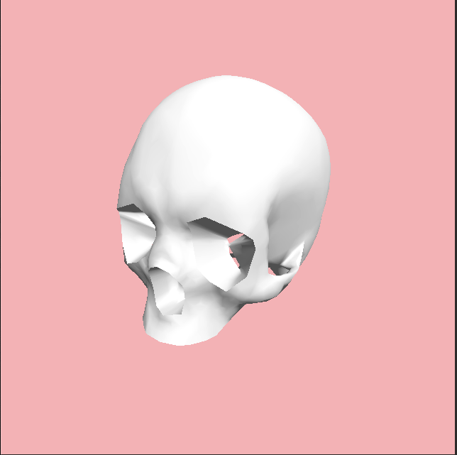
OBJ files are good for getting a simple 3D pipeline up and running. But, you
can outgrow the file format pretty quickly. File formats like FBX,
glTF, STEP,
or USD attempt to address OBJ shortcomings.
For my needs, I see a glTF importer in my future.
It’s great having the ability to leverage off the shelf tools for creating meshes. However, it’s just one capability. The workflow of building a landscape in a 3D editor, exporting it, and then importing it into my engine doesn’t get me to where I want to go.
I want the ability to create landscapes procedurally. My imagination gets going when I start to think about 3D worlds that could be dynamically changing while a simulation is running. This isn’t possible if I only enable a pipeline that uses external tools for mesh creation.
What’s the alternative?
I started exploring data structures that will support that long-term goal of procedurally generated meshes. To narrow down the possibilities I established a small list of requirements.
Landscape Requirements
- An agent can exist on a tile.
- A tile is a planer, convex polygon.
- Tiles can be joined at their edges to form landscapes.
- Complex geometries can be defined by changing the orientation of a tile.
To help keep things simple while starting out, I’m only focusing on uniform square tiles for the moment. With that in mind, what do I need to organize a bunch of tiles?
For starters, I need to know where each tile is in relation to each other. To do that, I established a coordinate system for a landscape. Using Euclidean space, a landscape has it’s ground plane defined by the X and Z axes and the Y axis specifies the elevation. For every point X, Y, Z; there may be zero or 1 tile.
I formalized the concept of a coordinate system with the Coordinate class.
# Coordinates can be in integers or floats, but we don't mix
# and match in the same landscape.
CoordinateType = TypeVar('CoordinateType', int, float)

class Coordinate(Generic[CoordinateType]):
  """
  A coordinate represents a location in a coordinate space.
  It can be of any number of dimensions (e.g. 1D, 2D, 3D,...ND)
  """
  def __init__(self, *components: CoordinateType) -> None:
    self._components = components

  # Skipping the rest of the class for brevity.
Can a landscape just be a collection of coordinates? Let’s try to create a procedurally generated landscape with just coordinates
import random
from agents_playground.spatial.coordinate import Coordinate

landscape_size_width: int = 10
landscape_size_length: int = 10
tiles: list[Coordinate] = []

# Distribute the tile elevations
tile_elevations: list[int] = random.choices(
  population=[0, 1, 2],
  weights=[10,2,1],
  k=landscape_size_width*landscape_size_length
)

# Create a tile for each spot in the XY plane.
tile_count = 0
for x in range(landscape_size_width):
  for z in range(landscape_size_length):
    tiles.append(Coordinate(x, tile_elevations[tile_count], z))
    tile_count += 1
This generates a list of tiles at locations that look something like this:
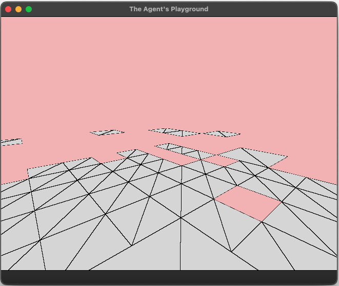
That’s not quite what I had in mind. I want the tiles to be connected and it’s clear that only using X,Y,Z coordinates won’t enable creating ramps or walls.
To expand on this idea, I started thinking about voxels. The basic concept is that a 3D mesh is represented by sections of 3D volumes. The volumes are usually cubes (think Minecraft) but they can be other shapes as well.
Voxels based rendering leads down two paths, volume rendering and mesh extraction. I’m currently going down the mesh extraction route. Algorithms such as marching cubes, surface nets, and dual contouring are established for creating meshes that represent isosurfaces.
Ultimately, I think a dual contouring approach is the the right answer for what I’m trying to achieve. Before doing that though, I’m working through establishing the primary architecture of the 3D engine. As a stop gap, I’ve implemented a poor man’s landscape topology.
Here is My Naive Approach
- Represent a 3D landscape as an infinite 3D lattice. The lattice is composed of uniform cubes.
- Each cube may contain zero or more tiles.
- Tiles may not occupy the same exact location.
- A tile may be placed in a cubes volume by connecting any two opposing edges. This rule enables creating tiles on any of the cube’s sides and also creating ramps or angled walls.
Given that there are a very short list of possible tile placements, these can be represented in a lookup table using enumerations.
from enum import IntEnum

class TileCubicPlacement(IntEnum):
  """
  Given a tile placed on an axis aligned cube, the
  TileCubicPlacement specifies which face of the volume
  the tile is on.

  Front/Back are on the X-axis.
  Top/Bottom are on the Y-axis.
  Left/Right are on the Z-axis.
  """
  # The Cube Sides
  FRONT  = 0
  BACK   = 1
  TOP    = 2
  BOTTOM = 3
  RIGHT  = 4
  LEFT   = 5

  # The Cube Diagonals.
  # These are used to create walls and ramps.
  # Diagonals are formed by defining a tile between
  # opposing edges. For example FB_UP is connection the the
  # Front Face to the Back Face by a tile from the lower edge
  # on the front face to the upper edge on the back face.
  FB_UP   = 6 # Front to Back, Lower Front Edge to Top Bottom
  FB_DOWN = 7 # Front to Back, Top Front Edge to Bottom Lower
  LR_UP   = 8 # Left to Right, Lower Left Edge to Top Right
  LR_DOWN = 9 # Left to Right, Top Left Edge to Bottom Right

  # Front to Back
  # Front Left Vertical Edge to Back Right Vertical Edge
  FB_LR   = 10

  # Front to Back
  # Front Right Vertical Edge to Back Left Vertical Edge.
  FB_RL   = 11
With this approach, a tile can be placed with a four part tuple for the form (X, Y, Z, TileCubicPlacement). The X, Y, and Z values are the coordinates of the cube in the lattice and the TileCubicPlacement value indicates where in the cube the tile is located.
This is clearing looking at an example. Here are the coordinates of a strip of tiles going up the X-axis with a ramp up and then ramp down.
tiles = [
  # Of the form (X, Y, Z, TileCubicPlacement)
  [0, 0, 0, 3], # Bottom Tile
  [1, 0, 0, 3],
  [2, 0, 0, 8], # Ramp Up
  [3, 1, 0, 3],
  [4, 1, 0, 3],
  [5, 0, 0, 9], # Ramp Down
  [6, 0, 0, 3],
  [7, 0, 0, 3]
]
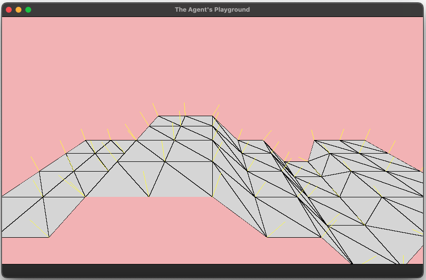
When rendered, the landscape looks like the below image. Note, the X-axis is going from
left to right in this image.
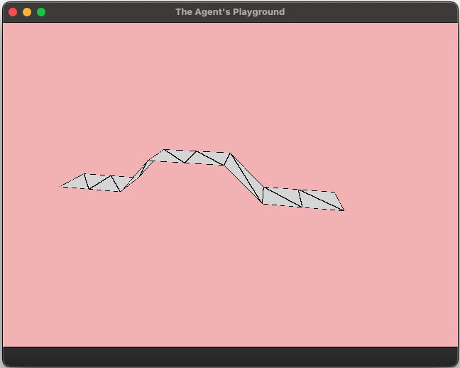
This is a pretty crude landscape solution but that’s ok. It’s just a stop gap solution while I prop up other parts of the engine. Speaking of which, let’s look at some of the other aspects of the landscape pipeline.
Landscapes on Disk#
With defining meshes established, I need a way to store a landscape on disk.
The original 2D engine uses TOML files for representing simulation scenes. TOML worked ok for small scenes but it isn’t robust enough for more complex scene. Additionally, that approach required a lot of code for verifying the correctness of the file when loading it into memory. For the 3D engine I decided to go back to the drawing board for how simulation scenes are organized.
This time around I decided to go with JSON files and use JSON Schema to define
the contracts for both a Scene file and a Landscape file. With this approach, a
scene consists of multiple files.
| File | Format | Description |
|---|---|---|
| scene | JSON | The top level file. Organizes all of the assets to be included in the simulation. |
| landscape | JSON | Responsible for defining a landscape. Is referred to by the scene file. |
| agent | JSON | Represents a conceptual model for an agent. Is referred to by the scene file. |
| model | OBJ, glTF | A 3d mesh. Can be referred to by agent and scene files. |
This is a step up from the TOML file approach. It’s easy to validate files with JSON Schema. However, parsing files produces a nested dictionary. This isn’t great for representing a 3D mesh.
Landscapes in Memory#
Now comes the hard part. How should the landscape be represented in memory as a mesh? Once the landscape is in memory it needs to be used for a variety of things. For example, agent navigation, collision detection, and rendering.
The answer is, there are several in-memory representations of the landscape.
Here is the current landscape data flow.
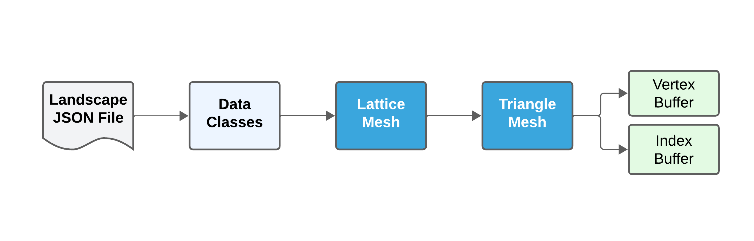
I use Python data classes for the initial representation of the landscape. This is done to simplify the code.
The JSON parser included in the Python standard library builds a dictionary when parsing JSON files. I convert this to a hierarchy of data classes to have a tighter definition of the various components. The conversation process is handled by by implementing the Dunder method __post_init__ on each data class.
from dataclasses import dataclasses

@dataclass
class Landscape:
  # Tiles are organized by their location for rapid lookup.
  tiles: dict[Coordinate, Tile]

  def __post_init__(self) -> None:
    """
    A landscape is loaded from a JSON file. When that happens a
    dict[str, Any] is passed into a Landscape instance like
    Landscape(**json_obj). To handle this correctly,
    The various landscape members need to be set correctly.
    """
    # If being set from JSON, then self.tiles will be a list
    # of list[Any]. Convert this to a dict[Coordinate, Tile]
    if isinstance(self.tiles, list):
      # Grab a reference to the tiles.
      tile_placements: list[list[int]] = self.tiles

      # Redefine the tiles as a dict[Coordinate, Tile].
      self.tiles: dict[Coordinate, Tile] = {}

      # Place all the tiles in the preferred format.
      for tile_placement in tile_placements:
        tile = Tile(location=Coordinate(*tile_placement))
        self.tiles[tile.location] = tile
Once the data is available as data classes it needs to be organized into a mesh. I use the half-edge data structure to represent meshes.
The implementation of the half-edge data structure is more complex than I want to go into in this article. I may document it in the future though.
The half-edge data structure is great for working with enclosed meshes. It enables easily traversing across a meshes vertices, edges, and faces.
We not done though. The lattice mesh tells us where there are tiles but we can’t render them directly. Remember, a tile is currently defined as a square. The GPU can only handle rendering triangles.
Landscapes on the GPU#
The 3D engine leverages WebGPU to work with the GPU. GPUs don’t know about geometric concepts like squares and triangles. To actually render a landscape a few more (big) steps are needed.
Making Triangles
After the lattice is organized into a half-edge mesh, I apply a fan tessellation
algorithm on it to produce a half-edge mesh of triangles.
class Tesselator(Protocol):
  @abstractmethod
  def tesselate(self, mesh: MeshLike):
    """Tessellates a mesh in place."""

class FanTesselator(Tesselator):
  """
  Implements a simple fan tessellation scheme.

  For each face, with N number of vertices, it picks the first
  vertex and then breaks the face into triangles by creating a
  fan with the first vertex as the fan origin.

  This is only appropriate for convex polygons and throws an
  error if the the polygon is not convex.
  """
  def tesselate(self, mesh: MeshLike):
    face: MeshFaceLike
    for face in mesh.faces:
      # Is the face a triangle? If so, skip.
      # Otherwise break into a fan.
      if face.count_boundary_edges() == 3:
        continue

      vertices: list[MeshVertexLike] = face.vertices()

      # Can a fan be constructed?
      # A fan can only be constructed on convex polygons.
      if not is_convex(vertices):
        raise tessellationException()

      fan_point = vertices[0]

      # Remove the face that is about to be
      # replaced with triangles.
      mesh.remove_face(face)

      # Loop over the vertices in the range [1:N-1]
      # Skipping the first and last vertices.
      for current_vert_index in range(1, len(vertices) - 1):
        mesh.add_polygon(
          vertex_coords = [
            fan_point.location,
            vertices[current_vert_index].location,
            vertices[current_vert_index + 1].location
          ],
          normal_direction = face.normal_direction
        )

  # Skipping the rest of the class for brevity.
This works for my poor man’s landscape topology but will be a bad fit for more sophisticated isosurface algorithms. In the future, I intend to replace this with a tessellation scheme that considers the entire mesh.
Generating Normals
The triangle mesh isn’t ready for rendering after it is initially created.
There are different ways to render things. The technique I’m using leverages shading models to calculate light intensity for every visible point on a 3D mesh.
The shading model is implemented in vertex and fragment shaders. To do their job, the shaders need the vertices of the mesh and their corresponding vertex normals. To do that, I need to calculate the vertex normal of every vertex in the triangle mesh.
The high level algorithm is:
- For each triangle calculate it’s face normal.
- For each vertex, calculate the vertex normal by taking the average of the adjacent face normals.
Finding a Face Normal
Here is how I calculate the face normals.
class HalfEdgeMesh(MeshLike)
  def calculate_face_normals(self, assume_planer=True) -> None:
    for face in self._faces.values():
      vertices = face.vertices()
      if assume_planer:
        # For polygons that are known to be planer, just take
        # the unit vector of the cross product.
        vector_a: Vector = vector_from_points(
          vertices[0].location,
          vertices[1].location
        )

        vector_b: Vector = vector_from_points(
          vertices[0].location,
          vertices[len(vertices) - 1].location
        )
        face.normal = vector_a.cross(vector_b).unit()
      else:
        # If we can't assume the polygons are planer, then use
        # Newell's method as documented in Graphic Gems III
        # (algorithm) and volume IV (Andrew Glassner's implementation).
        face.normal = self._newells_face_normal_algorithm(vertices)
  # Skipping the rest of the class...
It’s straightforward to calculate the vertex normals after the mesh’s face vector normals are known. For each vertex, I find all the faces that are connected to vertex and then calculate the average of the face normals.
Calculating a Vertex Normal
class HalfEdgeMesh(MeshLike):
  def calculate_vertex_normals(self) -> None:
    """
    Traverses every vertex in the mesh and calculates each
    normal by averaging the normals of the adjacent faces.
    Normals are stored on the individual vertices.
    """
    vertex: MeshVertexLike
    for vertex in self._vertices.values():
      # 1. Collect all of the normals of the adjacent faces.
      normals: list[Vector] = []

      def collect_normals(face: MeshFaceLike) -> None:
        if face.normal is None:
          # Attempted to access a missing normal on face.
          raise MeshException()
        normals.append(face.normal)

      num_faces = vertex.traverse_faces([collect_normals])

      # 2. Calculate the sum of each vector component (i, j, k)
      sum_vectors = lambda v,
        v1: vector(v.i + v1.i, v.j + v1.j, v.k + v1.k)
      normal_sums = functools.reduce(sum_vectors,  normals)

      # 3. Create a vertex normal by taking the average
      #    of the face normals.
      vertex.normal = normal_sums.scale(1/num_faces).unit()

  # Skipping the rest of the class...
Building Buffers
The last step in the landscape pipe is to produce a vertex buffer object
and vertex index object to pass to the GPU for rendering.
This sounds more complicated than it really is. A vertex buffer is just a linear array that has the vertices and any related data packed together. The index buffer is used to track how many vertices there are.
The vertex buffer is constructed by the SimpleMeshPacker class. The algorithm is to loop over all the triangles in the landscape mesh and pack each triangle’s vertices, texture coordinates, vertex normals, and Barycentric coordinates.
class SimpleMeshPacker(MeshPacker):
  """
  Given a half-edge mesh composed of triangles, packs a
  MeshBuffer in the order:
  Vx, Vy, Vz, Vw, Tu, Tv, Tw, Ni, Nj, Nk, Ba, Bb, Bc

  Where:
  - A vertex in 3D space is defined by Vx, Vy, Vz.
  - The related texture coordinates (stubbed to 0 for now) is
    defined by Tu, Tv, Tw.
  - The vertex normal is defined by Ni, Nj, Nk.
  - The Barycentric coordinate of the vertex is defined
    by Ba, Bb, Bc.
  """

  def pack(self, mesh: MeshLike) -> MeshBuffer:
    """Given a mesh, packs it into a MeshBuffer."""
    buffer: MeshBuffer = TriangleMeshBuffer()

    # Just pack the vertices and normals together to
    # enable quickly rendering.
    face: MeshFaceLike
    fake_texture_coord = Coordinate(0.0, 0.0, 0.0)

    for face in mesh.faces:
      vertices: list[MeshVertexLike] = face.vertices()
      for index, vertex in enumerate(vertices):
        bc = assign_bc_coordinate(index)
        buffer.pack_vertex(
          location = vertex.location,
          texture = fake_texture_coord,
          normal = vertex.normal, #type: ignore
          bc_coord = bc
        )

    return buffer

  # Skipping the rest of the class.
Wrapping Up#
And that’s it! The first pass on the landscape pipeline is complete. For the
0.2.0 version of the engine the goal is to get the major components in place.
I’m happy that I can now say that’s the case. A landscape can go from a JSON file
to pixels on the screen.
Things aren’t perfect. The landscape mesh extraction process is flakey. While the landscape protocol enables defining walls, the reality is that it’s very buggy. There are several tile combinations that can result in geometry that the half-edge mesh cannot represent. That’s ok. Baby steps.
While it’s not robust yet, the foundation is in place. In version 0.3.0, I intend to replace the current landscape algorithm with a robust isosurface algorithm. I’m also looking forward to building a landscape editor so defining landscapes by hand in a JSON file will become a thing of the past. Additionally, I’m keen to try shifting some of the CPU work to compute shaders.
But those are all challenges for another day.
Until next time…
- Sam